Future of Sun and Earth – A Scientific Animation
During my 5th semester of my Media and Communications Informatics Bachelor’s degree I got to lead a team of 15 talented fellow students. The end result was an animation of the future development of the Sun and it’s affects on the Earth, which can be seen here:
 🌍 Click here or on the image to see the full animation! ☀️
 In this post you can read a few chapters from the project documentation, that can be found in full (186 Pages) as an attachment at the bottom of this page. It details the whole research and animation process, broken down for each scene.
#1 Introduction
The given task was to create an animation showing the future development of the sun and the earth. The animation should start at the current time and end at the point of time, where the Sun as we know it today, ceases to exist and transitions into a planetary nebula. The simulation should show the transition of the Sun from its current status, to its increase in luminosity and size, to becoming a red giant, a white dwarf, and finally a planetary nebula. In addition, changes caused by that on the earth should be shown in the simulation.
The task stated above was the content of an interdisciplinary project, where students from different study programs work together on the same project. Each bachelor degree student of the Rhine-Waal University of applied sciences chooses and participates in a interdisciplinary project in the fifth semester. The participants of this interdisciplinary project are predominantly students from ‘Medien und Kommunikationsinformatik’, but also from the courses of ‘E-Government’, ‘Communication and Information Engineering’, ‘Digital Media’ and ‘Environment and Energy’. The diverse backgrounds were taken as an invitation to split the participants into two teams; One for research and one for graphics. The research team was responsible for finding the relevant data and presenting it to the graphics team to discuss together what happens, what is important to animate, how detailed it should be and what elements needed further research. The graphics team used the open source Blender program to create the individual elements and later on put them together in scenes
#2 Project Management
Antonio Sarcevic was voted as project lead on the 08.11.2018. A discord server was created to ensure that everyone in the group can communicate with each other. Trello is used as a kanban board to organize incoming tasks and multiple Google Drive files were created to track progress of the team and record the time spend on the project.
#4 Summary of the simulation
The simulation starts in the present-day with a fly-by of the earth showing the actual state of the planet. The Sun can be seen in the background. As time progresses, the greenhouse effect get stronger, and the climate on earth becomes more extreme. This is animated by a close-up of Earth’s surface showing strong rain and forest fires as examples of these conditions. The shift of the climate zones is visualized in the next scene from a viewpoint in space which shows the climate zones enlarging towards the poles. By 2050 the arctic and antarctic are expected to be ice free in summer. To represent this visually, the next scene is a split screen. One half shows a close up of melting ice, viewed from Earth’s surface, and the other half shows Earth from space to visualize the rising sea levels. As the luminosity of the Sun increases, the surface water of the Earth heats up and starts to boil and evaporate. This occurs around 1 billion years in the future. The evaporation of the water leads to further reactions in the atmosphere that change its composition. This results in a dense, Venus-like atmosphere which is shown from space. Eventually, the loss of Earth’s magnetic field leads to the loss of its atmosphere, leaving a brownish planet. For the next part of the simulation the focus shifts to the sun, which continues to grow in size and change colour. It progresses from white, to orange, and then to red while also increasing in luminosity. This all occurs as the sun progresses to a red giant. It continues to undergo various changes, including helium ignition and eventually hydrogen-exhaustion, as it progresses toward the end of the asymptotic-giant-branch, whereupon its core collapses into itself and becomes a white dwarf. While this is happening, its outer layers float away into space and form a planetary nebula, made visible with the help of radiation emitted by the white dwarf.
#5 Storyboard
Before initial research had begun, a simple storyboard was created to help visualize an overview of the project as well as to begin an exchange in the group as to what key points needed to be visualized, and how to best represent them. The first draft of the storyboard was created using free stock photos and altering them with photo editing software to achieve the desired look. Color changes were achieved by selecting the desired area to isolate, or selecting a specific color range, and then altering the color by either adjusting the color balance or using the replace color option if available. For the magma effect on the earth, a lava texture was placed on the layer above the earth and cut to the be the same shape as the earth. The layer was then set to overlay and some erasing of key areas was done to get the desired look.
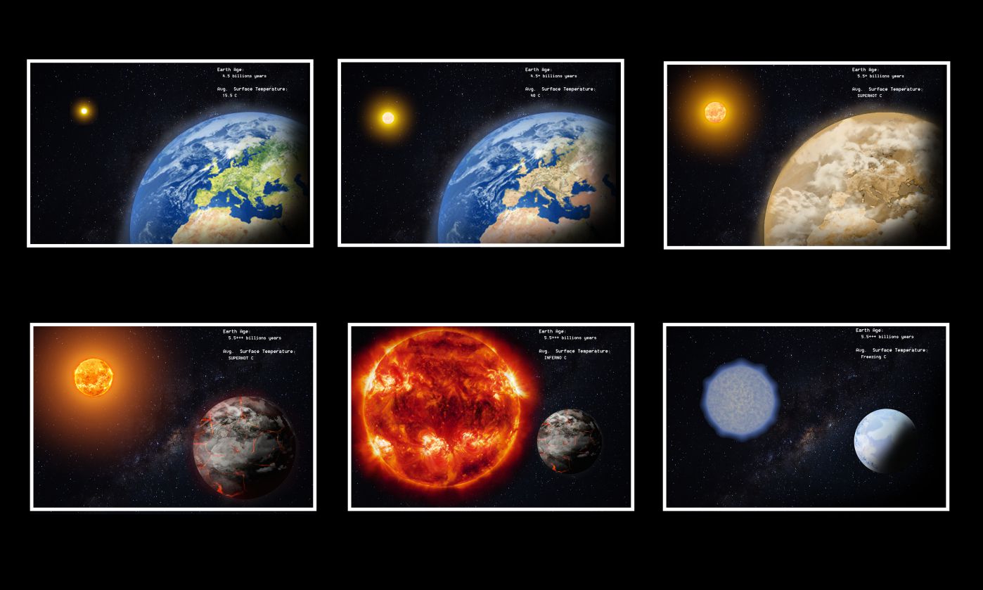
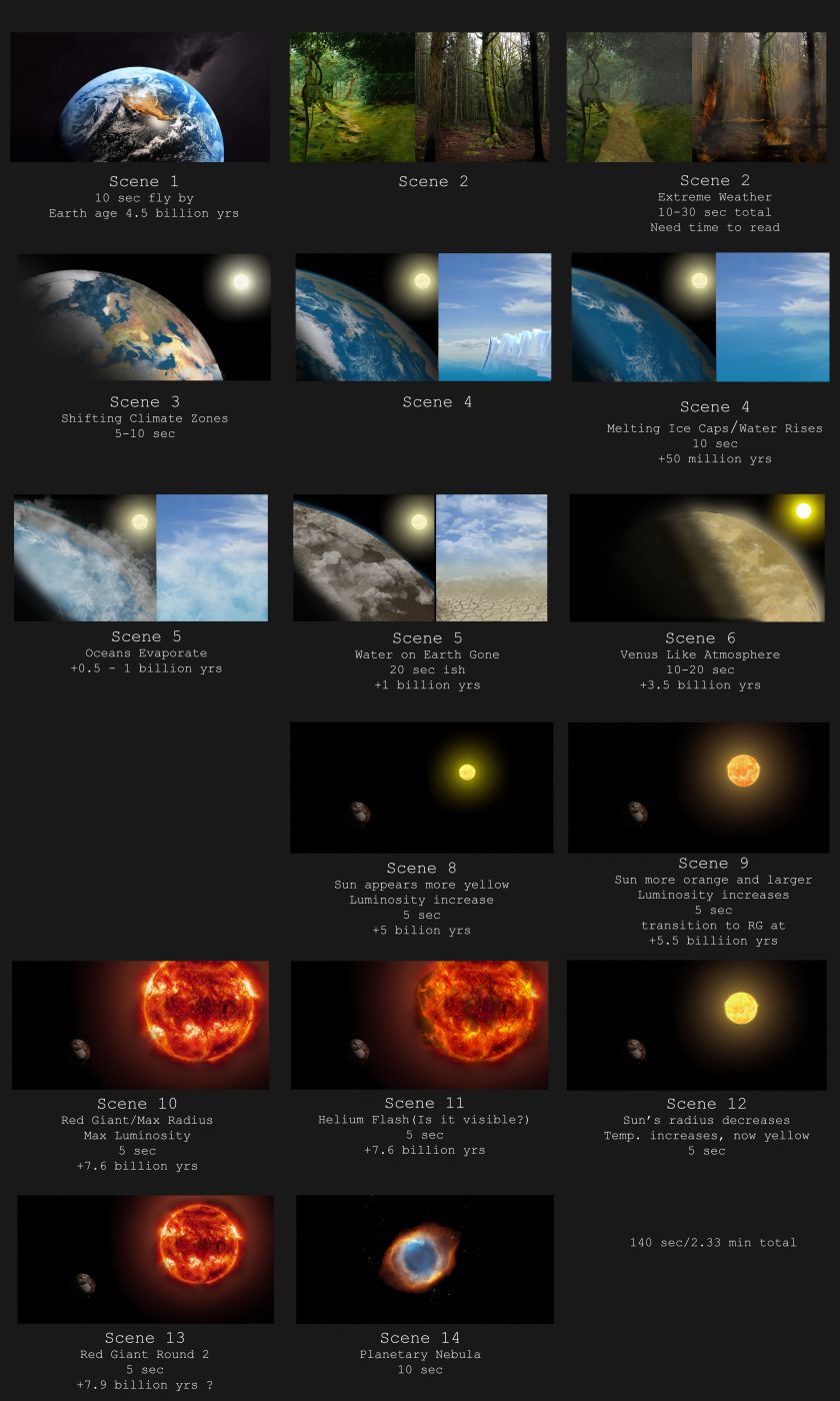
After research had been completed, a final storyboard was created to document the timeline of the animations and highlight key points, allowing the graphics team to easily visualize what needed to be modelled, and how the changes of the earth and sun would appear. As was done in the first version, photo manipulation was used to visualize the project, and to keep the ideas as clear as possible and close to what the final product would resemble. Fire and steam effects were created using free Photoshop brushes found on brusheezy.com and altering their opacity to generate the desired effect. Some further research needed to be conducted, in order to fill-in visual gaps. This made the final version of the storyboard as clear as possible for the graphics team. After the visual elements of the storyboard were confirmed by the research team as correct, time frames were calculated for each scene and important dates added to give an idea of how fast transitions should occur.
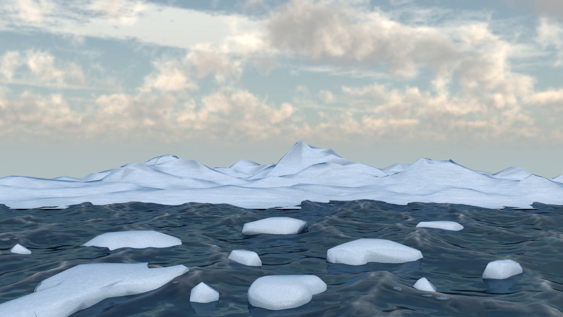
#9.2 Scene 4: melting ice caps, sea levels rising; Animation: Close-Up View
Antonio Sarcevic was responsible for creating the close-up view of Scene 4 in Blender. The steps needed to create this scene include finding and editing a fitting HDRI, creating an ocean plane with fitting settings and material, sculpting ice sheets and creating an ice material, creating an iceberg using Add-ons and animating the whole scene using keyframes.
#9.2.1 HDRI
For this Scene, an HDRI Image is used for the sky and clouds in the background. After finding a mostly fitting HDRI online, it still had to be edited to make it work for our scene. Opening up the HDRI in a raster graphics editor (here Photoshop was used) lets you edit the image directly. Use a selection tool to select the ocean from the HDRI because we don’t need it since we will add an animated ocean in Blender. Use a color picker to pick a fitting color to replace the ocean with. Choose a color near the horizon. To create a smooth transition from the sky to the missing ocean, select the gradient tool and choose a gradient between the chosen color and transparent. Zoom near the horizon and apply a gradient from where the ocean starts, to where the clouds start to be visible. Hold shift to make the gradient perfectly horizontal.
Save this image as a “.hdr”-File. Create a new Blender scene to insert the HDRI into. Important: at the top of the window set the Renderer to Cycles Render. In the Properties window select the World tab. Under Surface click the Use Nodes button. Open a Node Editor window and from the toolbar at the bottom select the World icon. Add an Environment Texture node by clicking Add from the bottom toolbar, then Texture and then Environment Texture. Connect the Color parameter from the Environment Texture node to the Color parameter from the Background node. Click the Open button and select the edited Texture. Rotating the HDRI is possible using a Mapping node connected to the Vector property of the Environment Texture node
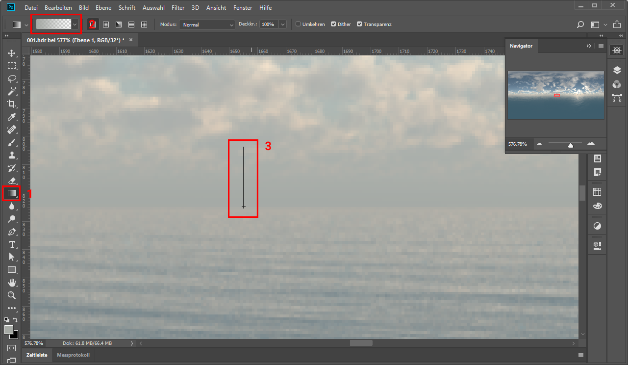
Create the gradient to replace the ocean in the HDRI. (1) Select the gradient tool. (2) Select a gradient from the picked color to transparent. (3) Click and drag from the ocean to the start of the clouds in the image.
To set up the camera select the Camera from the Outliner to edit its properties. In the 3D Viewport change the Location on the right-hand side to 0, -50, 10 and the Rotation to 90°, 0°, 0°. The Scaling can be set to 200, 200, 200 to get a better view of what the camera sees. Under the Properties window, select the Data tab and set the Clipping to Start at 1 and End at 240.
#9.2.2 Ocean
Start by adding a plane into the scene. To create a plane use the 3D Viewport in Object Mode and select Plane from the Create tab in the left-hand menu. The location can be changed in the right-hand menu of the 3D Viewport (press N to open it, if it isn’t open) and was set to -75, 0, 0. Rename the Plane to Ocean in the Outliner window.
After creating the plane, open the Modifiers tab in the Properties window. Click Add Modifier and select Ocean under Simulate. This opens up a range of options. First, make the ocean bigger by setting both Repeat X and Repeat Y to 4. Set the Resolution to 12 the Choppiness to 1.5. Alignment is set to 1. One can press the Bake Ocean button to bake the ocean for faster working later. Also important is to check the Generate Foam box and put in a name like “Foam” for the Foam Data Layer Name.
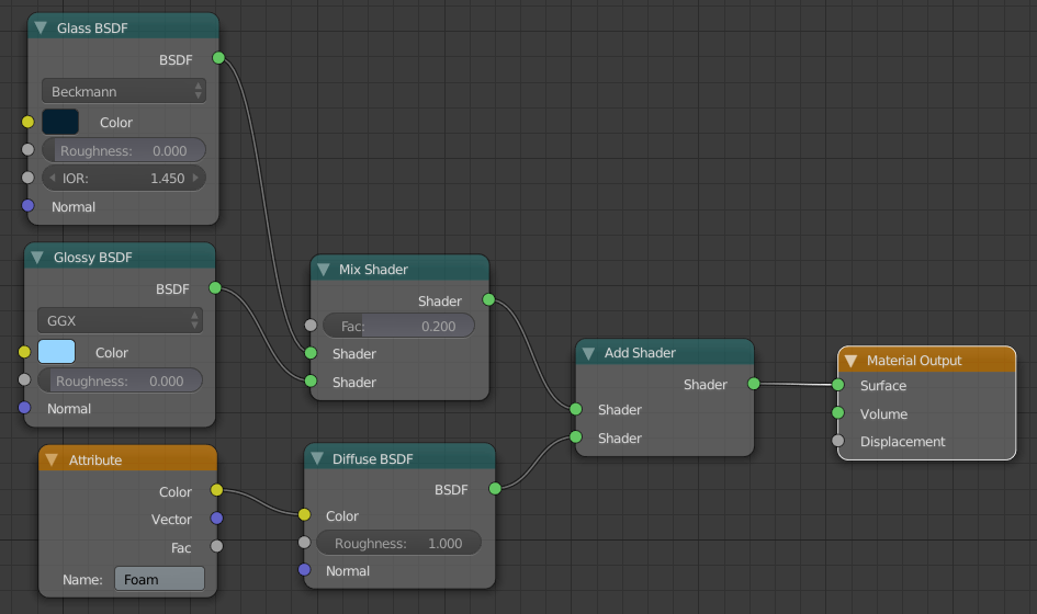
To create a material for the ocean plane, go to the Material tab in the Properties window and click New. Name the material Ocean and open up a Node Editor window to edit the material. To create a node press CTRL and A and click Search to search for the node names given. First, a Glass BSDF is added and set to Bleckmann with a dark blue color (HEX #052031). The roughness is set to 0 and the IOR is set to 1.45. Then a new Glossy BSDF is added with a light blue color (HEX #96D5FF). These both get plugged into a Mix Shader node with a factor of 0.2. Below, create a new Attribute node with the name you set in the Foam Data Layer Name before. This gets plugged into a Diffuse BSDF node with a Roughness of 1. The Mix Shader from above and the Diffuse BSDF from below both get plugged into an Add Shader node and this Add Shader node gets plugged into the Surface input of the Material Output node. Recreate this material by using CTRL and A to add the nodes and copy the values from the image.
#9.2.3 Ice sheets
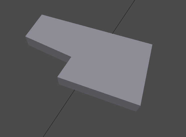
Start by creating a Cube in the Create tab of the Object Mode inside the 3D Viewport. Scale the Cube to a desired size of the ice sheet. Use the Numpad 0 key on the keyboard to view the scene from the camera’s perspective and determine a good location and size for the ice sheet. You can also rotate the cube to make the scene more varied. Rename the Cube to Ice in the Outliner window. Disable the Ocean layer by pressing the little eye icon in the Outliner so you can view your work better. Next, press the Numpad Comma / Period key to focus the camera on the cube.
To give the ice some shape, one can add another cube to carve out some parts of the original cube to give it some shape. After adding another cube, scaling it larger on the Z axis than the original cube and placing it where it should carve the ice select the original ice cube again.
With the ice cube selected go to the Modifiers tab in the Properties window, click Add Modifier and select Boolean under the Generative section. Under object select the newly made Ice block that we placed to carve the ice then under Operation set it to Difference and press Apply. Then go ahead and delete the new block.
One can repeat this progress to make unique shapes for the ice base. Then go to into the Sculpt Mode in the 3D Viewport and in the right-hand menu of the 3D Viewport select Matcap under Shading. In the left-hand menu of the 3D Viewport select the Scrape/Peaks tool and set the Radius to a desired size and the Strength to 1. Under Stroke set the Spacing to 1%. Under Curve select the flat curve (the last button under the graph view). And be sure to have a checkbox in the Dyntopo setting. Also uncheck every axis in the Symmetry/Lock feature. Then go ahead and hold your left mouse button and move it over the edges of the ice base to shape it into a desired model. Experiment with different radii and camera views to get different results. Scrape the ice sheet base into a general ice shape. Smooth out the corners and give it the desired look. Use Ctrl + Z to undo undesired changes. This part requires a lot of trial and error. If you want to add material to work with use the Blob or Clay tool to add more material. You can use the Smooth tool to fix mistakes or generally smooth the surface more, but a more “edged” look is more desirable.
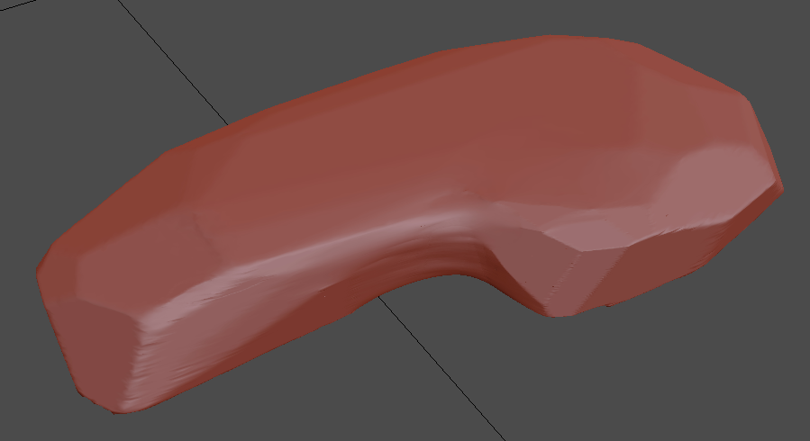
Apply sculpting the object, leave Sculpt Mode and go back to Object Mode. After creating several ice sheets with different sizes and shapes, place them in the scene, copy and rotate some to fill the lower half of the ocean. Matcap can be also disabled now. To finish up the ice sheet, one should decrease the complexity of the mesh. To do this go to the Property window and select the Modifier tab. Click on Add Modifier and select the Decimate modifier. Lower the ratio until the Faces reach a number between about 100 and 1000.
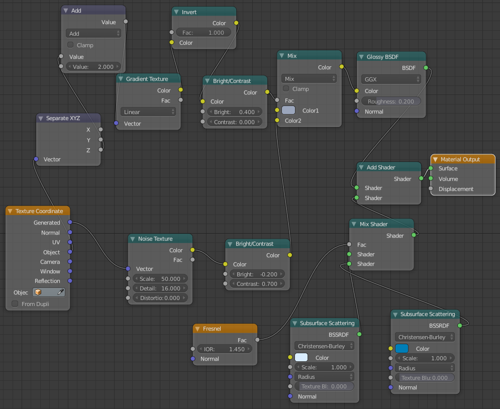
Create a new material like described above. Name it Ice and add a Texture Coordinate node. Plug the Object output into a Separate XYZ node. Plug the Z output into a Math node and set it to Add and set the other value to 2. This output gets plugged into a Gradient Texture node set to Linear. This output gets plugged into an Invert node and this output gets plugged into a Bright Contrast node with a Bright of 0.4 and Contrast set to 0. Go back to the Texture Coordinate node and plug the Generated output into a new Noise Texture node with Scale set to 50, Detail set to 16 and Distortion set to 0. The Color output gets plugged into a Bright Contrast node with a Bright of -0.2 and Contrast of 0.7. The last Bright Contrast node gets plugged into the Color 2 of a MixRGB node and the Bright Contrast form before gets plugged into the Fac of the same MixRGB node. The Color1 of the MixRGB gets set to a greyish blue (HEX #9BA6BC). This MixRGB node gets plugged into a Glossy BSDF with a roughness of 0.2. Go below and create a Fresnel node with IOR of 1.45. Create two Subsurface Scattering nodes with one being blueish almost white (HEX #D9EDFF) and the other a more vibrant blue (HEX #007EB7). Create a Mix Shader node and plug the Fresnel Fac into the Fac of Mix Shader and the Subsurface Scattering in both Shader inputs of the Mix Shader. This last Mix Shader and the Glossy BSDF from above both get plugged into an Add Shader and this gets plugged into the Surface input of the Material Output.
#9.2.4 Iceberg
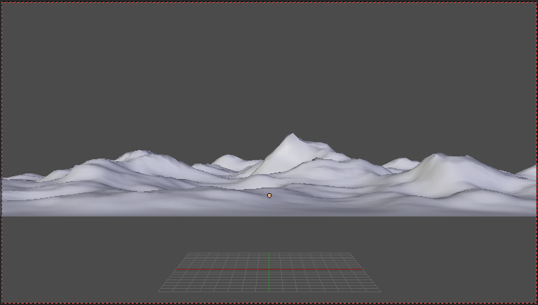
In the background an iceberg will be added. To generate a mountain structure we will use a Blender Add-on. To enable the plugin go to File then User Preferences then select the Add-ons tab. Search for “Landscape” and check the box next to “Add Mesh: A.N.T.Landscape” and click Save User Settings.
After enabling the add-on there will be a new option under the Create tab of the Object Mode. Below the Add Primitive section there is a Landscape section with a Landscape button. Click the button to add a new landscape. On the left hand side there also will be a new section at the bottom (or press the little plus icon if it is missing) called “Another Noise Tool - Landscape”. This section contains all the settings for the newly added landscape mesh. Use the Mesh Size X and Mesh Size Y to scale it to the desired size. Under Noise Settings select Slick Rock as a Noise Type. To make the mountains bigger set the Maximum and Height to a larger value under the Displace Settings. To decrease the amount of pointy mountains set the Noise Size to a higher value. The Offset X/Y and Size X/Y of the Noise Settings can be manipulated to create different effects. Play around with the settings until there is a desired result. Add the ice material used in the ice sheets.
This part of the scene is based off the beginning of the Tutorial “Blender Tutorial- Create Realistic Mountains Free”. View this video for further details.
#9.2.5 Keyframe animation
First set the total length of the animation. Open up the Render tab inside the Property window and under Dimensions set the Resolution to X: 1920 and Y: 1080. Under Frame Range set the Start Frame to 1 and End Frame to 260.
Next up is animating the ocean. Note the Time parameter inside the Ocean Modifier. This needs to be animated for the ocean to simulate movement. To add a keyframe, be sure that in the Timeline the Current Frame is set to 0, then hover over the Time parameter of the Ocean modifier and press the I key on the keyboard. Then go to the last frame of the animation and set the Time to 20 and press I again. To animate the ocean level rising create a keyframe on the Location of the Ocean plane at Time 10. Go to the end of the animation, rise up the ocean as much as you like and create another keyframe on the Location. Opening the Graph Viewer allows the user to set curves for the animations. To create a smooth slow-then-fast rising water, adjust the curves in the Graph Viewer.
To animate all the ice sheets and the iceberg go to Time 10, select them all from the Outliner with Shift held down, then head to the 3D View and click Object from the bottom toolbar, then Animation, then Insert Keyframe and then select Scaling. Then go to the end of the animation and change the scale of all objects to 0 by holding ALT while clicking on Scale Z and typing in 0. Then add another keyframe through Object, Animation, Insert Keyframe and then Scaling.
Thanks for reading this blog entry. Be sure to check out the entire animation and if you are interested you can read more in the Project Documentation attached below!
#Final Results
🌍 Click here or on the image to see the full animation! ☀️